Introduction to using The Tractor¶

The Tractor is a code for optimizing or sampling from models of astronomical objects. The approach is generative: given astronomical sources and a description of the image properties, the code produces pixel-space estimates or predictions of what will be observed in the images. We use this estimate to produce a likelihood for the observed data given the model: assuming our model space actually includes the truth (it doesn’t, in detail), then if we had the optimal model parameters, the predicted image would only differ from the actually observed image by noise. Given a noise model of the instrument and assuming pixelwise independent noise, the log-likelihood is just the negative chi-squared difference: (image - model) / noise.

To actually use the Tractor code to infer the properties of astronomical objects in your images, you will probably have to write a driver script, which will read in your data of interest, create tractor.Image objects describing your images, and source objects describing the astronomical sources of interest. The Tractor does not (at present) create sources itself; you have to initialize it with reasonable guesses about the objects in your images.

tractor.Image objects carry the data, per-pixel noise sigma (we: usually work with inverse-variance), and a number of calibration parameters. These include the PSF model, astrometric calibration (WCS), photometric calibration, and sky background model. Each of these calibrations can be parameterized and its parameters fit alongside the properties of the astronomical sources.

Sources, positions, and brightnesses¶

tractor.Source objects are rather nebulously defined, as we will see: below. A simple example is the tractor.PointSource class, which has a “position” and a “brightness”. A Source object must be able to render its appearance in a given tractor.Image; that is, is must be able to produce a pixel-space model of what it would look like in the given image. To do this, it must use the image’s calibration objects to convert the source’s representation of its position into pixel space (via the image’s WCS), convert its representation of its brightness into pixel counts (via the image’s photometric calibration or “photoCal”). It also needs the image’s PSF model.

The core Tractor code does not know or care about the exact types (python classes) you use to represent the position and brightness. The only requirement for a “position” or “brightness” class is that it have the right “duck type”, and that the image’s PhotoCal or WCS objects can convert it to image space. That is, the class you use for the “position” of sources must match the class you use for the “WCS” of the images, and the “brightness” of the sources must match the “PhotoCal” of the images. Let’s see an example to clarify this.

In this example, we are working in pixel space and raw counts; we use the PixPos class to represent pixel positions, and the Flux class to represent the image counts. We can then use the “null” calibration classes, which just pass through the position and flux values unmodified.

from tractor import *

source = PointSource(PixPos(17., 27.4), Flux(23.9))

photocal = NullPhotoCal()
wcs = NullWCS()

counts = photocal.brightnessToCounts(source.getBrightness())
x,y = wcs.positionToPixel(source.getPosition())
print 'source', source
print 'counts', counts, 'x,y', x,y

Which prints:

source PointSource at pixel (17.00, 27.40) with Flux: 23.9
counts 23.9 x,y 17.0 27.4

Instead, we could chose to work in RA,Dec coordinates, so we would use the RaDecPos class to represent the positions of sources in celestial coordinates, and one of the WCS calibration classes that expect celestial coordinates. Similarly, we could decide to work with brightness represented in Mags, and use a MagsPhotoCal.

from tractor import *
from astrometry.util.util import Tan

source = PointSource(RaDecPos(42.3, 9.7), Mags(r=12., i=11.3))

photocal = MagsPhotoCal('r', 22.5)
wcs = FitsWcs(Tan(42.0, 9.0, 100., 100., 0.1, 0., 0., 0.1, 200., 200.))

counts = photocal.brightnessToCounts(source.getBrightness())
x,y = wcs.positionToPixel(source.getPosition())

print 'source', source
print 'photocal', photocal
print 'wcs', wcs
print 'counts', counts, 'x,y', x,y

Which prints:

source PointSource at RaDecPos: RA, Dec = (42.30000, 9.70000) with Mags: i=11.3, r=12
photocal MagsPhotoCal(band=r, zp=22.500)
wcs FitsWcs: x0,y0 0.000,0.000, WCS TAN: crpix (100.0, 100.0), crval (42, 9), cd (0.1, 0, 0, 0.1), image 200 x 200
counts 15848.9319246 x,y 101.957357071 106.001652903

Notice a few things here: we created a Mags object with r and i-band mags. Then when we created the photocal, we told it that this image is r band. The Tractor doesn’t care how many parameters you use to represent your brightness, all it cares is that your PhotoCal class can convert it to counts. You could imagine representing a star’s brightness in terms of angular diameter and black-body temperature, and have your PhotoCal integrate its spectrum through a filter curve.

In this example, we gave the source magnitudes in two different bands. If we had, say, an image in each band, we count then fit its position and flux in both bands. The position (in RA,Dec) would be fit to jointly optimize the likelihood in the two images, while the fluxes would be fit independently of each other. The r-band image would just have nothing to say about the i-band magnitude, and vice versa.

In the Tractor code, the “duck types” are defined in the file tractor/ducks.py. This code is not actually used, it is just documentation written in code. A toolbox of typical choices for position and brightness and their corresponding WCS and PhotoCal are given in the file tractor/basics.py.

Parameters¶

Before going any further, let’s look at some of the infrastructure for how the Tractor deals with parameters. In the Tractor code, most objects (sources, image calibration objects) must be Params duck-type objects. That is, a source should act like a Params object, as should a PhotoCal object. The most important function calls are shown here:

>>> from tractor import *
>>> pos = RaDecPos(42.3, 9.7)
>>> print pos
RaDecPos: RA, Dec = (42.30000, 9.70000)
>>> print pos.getParams()
[42.3, 9.7]
>>> print pos.getParamNames()
['ra', 'dec']
>>> print pos.getStepSizes()
[0.00010145038861680802, 0.0001]
>>> pos.setParams([42.7, 9.3])
>>> print pos
RaDecPos: RA, Dec = (42.70000, 9.30000)
>>> pos.setParam(1, 10.0)
>>> print pos
RaDecPos: RA, Dec = (42.70000, 10.00000)

Most of the Tractor’s infrastructure for dealing with params is in the tractor/utils.py file, which is not easy reading. The hope, however, is that the resulting API is flexible and easy to use.

We often want to “compose” objects out of sub-objects (a PointSource has a position and a brightness), so there is a class for that, called MultiParams. It is also nice to be able to parameters or sub-objects by name; this is accomplished by the NamedParams mix-in class, though you’ll probably never have to use that in your own code. For example:

>>> from tractor import *
>>> source = PointSource(RaDecPos(42.3, 9.7), Mags(r=99.9))
>>> print source
PointSource at RaDecPos: RA, Dec = (42.30000, 9.70000) with Mags: r=99.9
>>> print source.pos
RaDecPos: RA, Dec = (42.30000, 9.70000)
>>> print source.brightness
Mags: r=99.9
>>> print source.pos.ra
42.3
>>> print source.brightness.r
99.9
>>> print source.getParams()
[42.3, 9.7, 99.9]
>>> print zip(source.getParamNames(), source.getParams())
[('pos.ra', 42.3), ('pos.dec', 9.7), ('brightness.r', 99.9)]

Notice that source.getParams() just concatenates the getParams() results from its pos and brightness sub-objects. This is a really general theme in the Tractor. A Tractor Image object is composed of all its calibration sub-objects; Image.getParams() gives a full description of the calibration parameters of the image. Similarly, a Tractor Catalog is a list-like container of sources whose getParams() method just concatenates the getParams() of all the source it contains. Taking this one step further, a Tractor object itself is composed of Images and a Catalog.

Thawing/Freezing Params¶

A powerful feature of the Tractor is that you can “freeze” a subset of the parameters – hold them fixed and exclude them from fitting. This power comes at a price, though (doesn’t it always?); freezing the right parameters can be a bit tricky, and objects with frozen parameters might not always act the way you expect.

For MultiParams objects, you can freeze and thaw sub-objects by name. A parameter is considered “thawed” if the full path from the Tractor object to the parameter is thawed.

One possibly surprising thing about frozen parameters is that they disappear from the getParams() and getParamNames() lists; they are also not counted in numberOfParams(), and setParams() will skip past them. Frozen parameters effectively disappear from view:

>>> from tractor import *
>>> cat = Catalog(PointSource(RaDecPos(42.3, 9.7), Mags(r=99.9)))
>>> print cat
Catalog: 1 sources, 3 parameters
>>> print zip(cat.getParamNames(), cat.getParams())
[('source0.pos.ra', 42.3), ('source0.pos.dec', 9.7), ('source0.brightness.r', 99.9)]
>>> cat[0].freezeParam('pos')
>>> print zip(cat.getParamNames(), cat.getParams())
[('source0.brightness.r', 99.9)]

Here we froze the “pos” sub-object of the PointSource, so it disappears from view. We could thaw the position, but then freeze its RA component:

>>> cat[0].thawParam('pos')
>>> cat[0].pos.freezeParam('ra')
>>> print zip(cat.getParamNames(), cat.getParams())
[('source0.pos.dec', 9.7), ('source0.brightness.r', 99.9)]

Handy functions include:

>>> cat.thawAllRecursive()
>>> print zip(cat.getParamNames(), cat.getParams())
[('source0.pos.ra', 42.3), ('source0.pos.dec', 9.7), ('source0.brightness.r', 99.9)]
>>> cat.freezeAllRecursive()
>>> cat.thawPathsTo('r')
True
>>> print zip(cat.getParamNames(), cat.getParams())
[('source0.brightness.r', 99.9)]
>>> print 'Thawed(self)   Thawed(parent)   Param', '\n', '-'*50
>>> for param, tself, tparent in cat.getParamStateRecursive():
...     print '   %5s      %5s           ' % (tself, tparent), param
Thawed(self)   Thawed(parent)   Param
--------------------------------------------------
    True       True            source0
   False       True            source0.pos
   False      False            source0.pos.ra
   False      False            source0.pos.dec
    True       True            source0.brightness
    True       True            source0.brightness.r

The last table shows that the freezeAllRecursive() call froze both the source pos but also pos.ra and pos.dec; just thawing pos won’t cause ra and dec to become active again; we have to thaw the full path down to ra and dec:

>>> cat[0].thawParam('pos')
>>> cat.printThawedParams()
source0.brightness.r = 99.9
>>> cat[0].pos.thawAllParams()
>>> cat.printThawedParams()
source0.pos.ra = 42.3
source0.pos.dec = 9.7
source0.brightness.r = 99.9

Optimization / Fitting¶

So far we haven’t actually created a Tractor object or fit anything. Time to get down to business.

As an example, let’s create a synthetic image manually, and then use the Tractor to fit a source model to it.

import numpy as np
import pylab as plt
from tractor import *

# Size of image, centroid and flux of source
W,H = 25,25
cx,cy = 12.8, 14.3
flux = 12.
# PSF size
psfsigma = 2.
# Per-pixel image noise
noisesigma = 0.01
# Create synthetic Gaussian star image
G = np.exp(((np.arange(W)-cx)[np.newaxis,:]**2 +
            (np.arange(H)-cy)[:,np.newaxis]**2)/(-2.*psfsigma**2))
trueimage = flux * G/G.sum()
image = trueimage + noisesigma * np.random.normal(size=trueimage.shape)

# Create Tractor Image
tim = Image(data=image, invvar=np.ones_like(image) / (noisesigma**2),
            psf=NCircularGaussianPSF([psfsigma], [1.]),
            wcs=NullWCS(), photocal=NullPhotoCal(),
            sky=ConstantSky(0.))

# Create Tractor source with approximate position and flux
src = PointSource(PixPos(W/2., H/2.), Flux(10.))

# Create Tractor object itself
tractor = Tractor([tim], [src])

# Render the model image
mod0 = tractor.getModelImage(0)
chi0 = tractor.getChiImage(0)

# Plots
ima = dict(interpolation='nearest', origin='lower', cmap='gray',
           vmin=-2*noisesigma, vmax=5*noisesigma)
imchi = dict(interpolation='nearest', origin='lower', cmap='gray',
             vmin=-5, vmax=5)
plt.clf()
plt.subplot(2,2,1)
plt.imshow(trueimage, **ima)
plt.title('True image')
plt.subplot(2,2,2)
plt.imshow(image, **ima)
plt.title('Image')
plt.subplot(2,2,3)
plt.imshow(mod0, **ima)
plt.title('Tractor model')
plt.subplot(2,2,4)
plt.imshow(chi0, **imchi)
plt.title('Chi')
plt.savefig('1.png')

# Freeze all image calibration params -- just fit source params
tractor.freezeParam('images')

# Save derivatives for later plotting...
derivs = tractor.getDerivs()

# Take several linearized least squares steps
for i in range(10):
    dlnp,X,alpha = tractor.optimize()
    print 'dlnp', dlnp
    if dlnp < 1e-3:
        break

# Get the fit model and residual images for plotting
mod = tractor.getModelImage(0)
chi = tractor.getChiImage(0)
# Plots
plt.clf()
plt.subplot(2,2,1)
plt.imshow(trueimage, **ima)
plt.title('True image')
plt.subplot(2,2,2)
plt.imshow(image, **ima)
plt.title('Image')
plt.subplot(2,2,3)
plt.imshow(mod, **ima)
plt.title('Tractor model')
plt.subplot(2,2,4)
plt.imshow(chi, **imchi)
plt.title('Chi')
plt.savefig('2.png')

# Plot the derivatives we saved earlier
def showpatch(patch, ima):
    im = patch.patch
    h,w = im.shape
    ext = [patch.x0,patch.x0+w, patch.y0,patch.y0+h]
    plt.imshow(im, extent=ext, **ima)
    plt.title(patch.name)
imderiv = dict(interpolation='nearest', origin='lower', cmap='gray',
               vmin=-0.05, vmax=0.05)
plt.clf()
plt.subplot(2,2,1)
plt.imshow(mod0, **ima)
ax = plt.axis()
plt.title('Initial Tractor model')
for i in range(3):
    plt.subplot(2,2,2+i)
    showpatch(derivs[i][0][0], imderiv)
    plt.axis(ax)
plt.savefig('3.png')

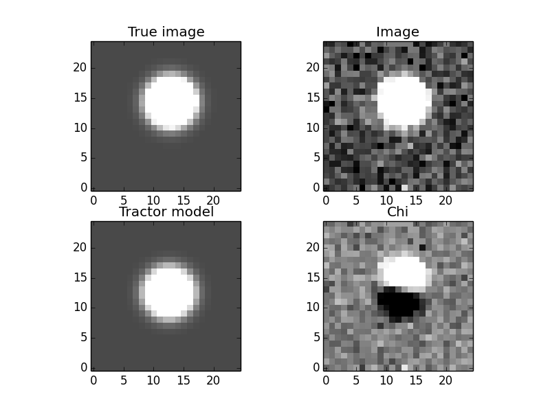
The plots look like:

The “before” image—our initial Tractor model has the source a little too low and to the left, which you can see in the “chi” image.

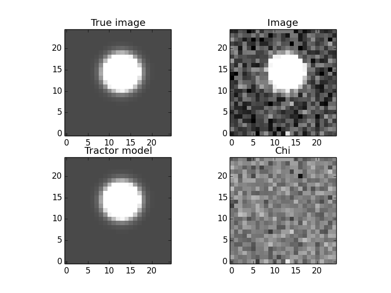
The “after” image—the source position has been adjusted and the “chi” image looks like a noise field.

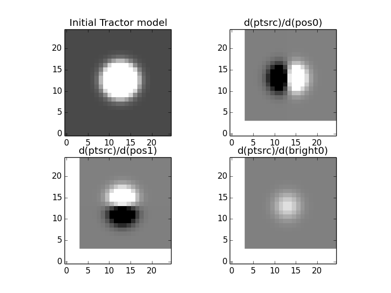
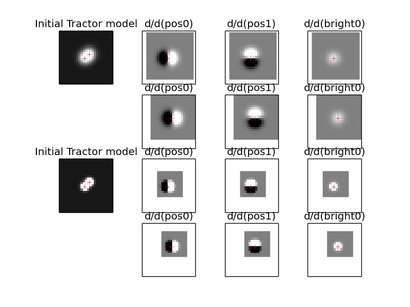
The “derivatives” image—the initial model, and its derivatives with respect to each of the parameters being fit. The fitter finds a linear combination of the derivatives that should minimize the residuals, then does line-search (since the minimum in the linearized problem may not coincide with the minimum in the real non-linear problem).

Multi-Image Optimization / Fitting¶

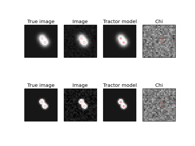
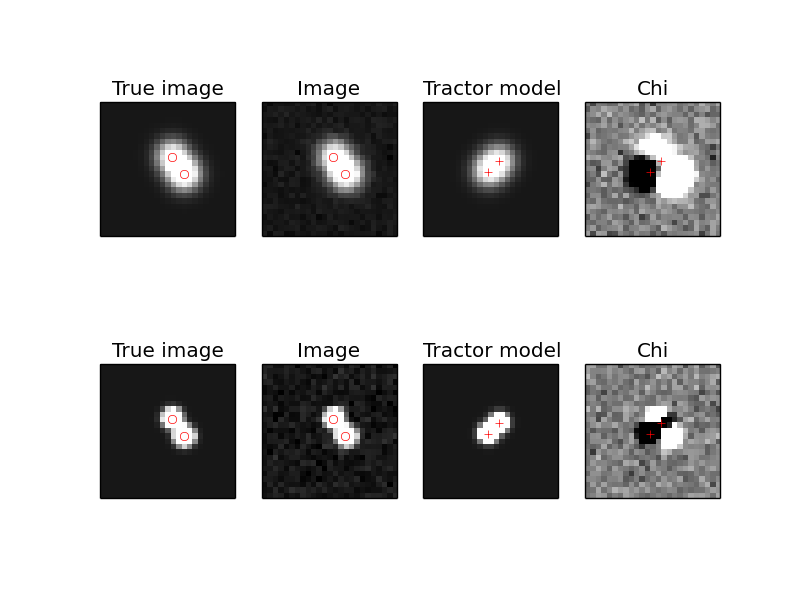
In the following example we will fit for the positions and fluxes of two point sources in two images with different point-spread functions and noise properties. The sources are within a few pixels of each other, so this is actually not a trivial problem for most source extraction routines, while for the Tractor the code is nearly identical to the easier single-image, single-source case.

import numpy as np
import pylab as plt
from tractor import *

def imshow(x, **kwa):
    plt.imshow(x, **kwa)
    plt.xticks([]); plt.yticks([])

# Size of image, centroids and fluxes of sources
W,H = 25,25
stars = [((12.8, 14.3), 12.), ((15.0, 11.0), 15.)]
# PSF sizes
psfsigmas = [2., 1.]
# Per-pixel image noise
noisesigmas = [0.01, 0.02]
# Create synthetic Gaussian star images
trueimages = []
images = []
for psfsigma, noisesigma in zip(psfsigmas, noisesigmas):
    trueimage = np.zeros((H,W))
    for (cx,cy),flux in stars:
        G = np.exp(((np.arange(W)-cx)[np.newaxis,:]**2 +
                    (np.arange(H)-cy)[:,np.newaxis]**2)/(-2.*psfsigma**2))
        trueimage += flux * G/G.sum()
    image = trueimage + noisesigma * np.random.normal(size=trueimage.shape)
    trueimages.append(trueimage)
    images.append(image)

# Create Tractor Images
tims = [Image(data=image, invvar=np.ones_like(image) / (noisesigma**2),
              psf=NCircularGaussianPSF([psfsigma], [1.]),
              wcs=NullWCS(), photocal=NullPhotoCal(),
              sky=ConstantSky(0.))
              for image, noisesigma, psfsigma
              in zip(images, noisesigmas, psfsigmas)]

# Create Tractor sourcess with approximate position and flux
cat = [PointSource(PixPos(W/2.-1, H/2.-1), Flux(10.)),
       PointSource(PixPos(W/2.+1, H/2.+1), Flux(10.))]

# Create Tractor object itself
tractor = Tractor(tims, cat)

# Render the model images
mods0 = [tractor.getModelImage(i) for i in range(2)]
chis0 = [tractor.getChiImage(i)   for i in range(2)]

# Plots
ima = dict(interpolation='nearest', origin='lower', cmap='gray',
           vmin=-2*noisesigma, vmax=20*noisesigma)
imchi = dict(interpolation='nearest', origin='lower', cmap='gray',
             vmin=-5, vmax=5)
def plot_src_pos(srcs):
    ax = plt.axis()
    plt.plot([src.getPosition().x for src in srcs],
             [src.getPosition().y for src in srcs], 'r+')
    plt.axis(ax)
def plot_true_pos(stars):
    ax = plt.axis()
    plt.plot([cx for (cx,cy),flux in stars],
             [cy for (cx,cy),flux in stars], 'o', mec='r', mfc='none')
    plt.axis(ax)

plt.clf()
for i,(trueim,im,mod,chi) in enumerate(zip(trueimages,images,mods0,chis0)):
    plt.subplot(2,4, 4*i+1)
    imshow(trueim, **ima)
    plot_true_pos(stars)
    plt.title('True image')
    plt.subplot(2,4, 4*i+2)
    imshow(im, **ima)
    plot_true_pos(stars)
    plt.title('Image')
    plt.subplot(2,4, 4*i+3)
    imshow(mod, **ima)
    plot_src_pos(cat)
    plt.title('Tractor model')
    plt.subplot(2,4, 4*i+4)
    imshow(chi, **imchi)
    plot_src_pos(cat)
    plt.title('Chi')
plt.savefig('4.png')

# Freeze all image calibration params -- just fit source params
tractor.freezeParam('images')

# Plot derivatives...
derivs = tractor.getDerivs()
def showpatch(patch, ima):
    im = patch.patch
    h,w = im.shape
    ext = [patch.x0-0.5,patch.x0+w-0.5, patch.y0-0.5,patch.y0+h-0.5]
    imshow(im, extent=ext, **ima)
    plt.title(patch.name.replace('d(ptsrc)', 'd'))
imderiv = dict(interpolation='nearest', origin='lower', cmap='gray',
               vmin=-0.05, vmax=0.05)
plt.clf()
for i,mod0 in enumerate(mods0):
    plt.subplot(4,4, 8*i+1)
    imshow(mod0, **ima)
    plot_src_pos(cat)
    ax = plt.axis()
    plt.title('Initial Tractor model')
    for j in range(6):
        plt.subplot(4,4, 8*i + (j/3)*4 + j%3 + 2)
        showpatch(derivs[j][i][0], imderiv)
        plt.axis(ax)
        plot_src_pos([cat[j/3]])
plt.savefig('5.png')

# Take several linearized least squares steps
for i in range(10):
    dlnp,X,alpha = tractor.optimize()
    print 'dlnp', dlnp
    if dlnp < 1e-3:
        break

# Get the fit model and residual images for plotting
mods = [tractor.getModelImage(i) for i in range(2)]
chis = [tractor.getChiImage(i)   for i in range(2)]
# Plots
plt.clf()
for i,(trueim,im,mod,chi) in enumerate(zip(trueimages,images,mods,chis)):
    plt.subplot(2,4, 4*i+1)
    imshow(trueim, **ima)
    plot_true_pos(stars)
    plt.title('True image')
    plt.subplot(2,4, 4*i+2)
    imshow(im, **ima)
    plot_true_pos(stars)
    plt.title('Image')
    plt.subplot(2,4, 4*i+3)
    imshow(mod, **ima)
    plot_src_pos(cat)
    plot_true_pos(stars)
    plt.title('Tractor model')
    plt.subplot(2,4, 4*i+4)
    imshow(chi, **imchi)
    plot_src_pos(cat)
    plt.title('Chi')
plt.savefig('6.png')