Using the Tractor with GalSim images

In the example below, we will process images generated by a modified version of the GalSim demo12.py script (Original: https://github.com/GalSim-developers/GalSim/blob/master/examples/demo12.py ; Modified: https://github.com/dstndstn/tractor/blob/master/doc/galsim/demo12.py).

Using the Tractor with GalSim images requires creating a tractor.Image object and source (PointSource, Galaxy) objects describing the objects in your scene.

Let’s start with the Image. For some experiments you would like to have the Tractor figure out the PSF itself, but here we will assume you want to tell it the true PSF model that was used. If you used a single Gaussian PSF in GalSim, that would look like:

from tractor import *
psf = NCircularGaussianPSF([sigma], [1.])

Be careful about PSF widths specified as full-width at half max (FWHM), or specified in arcseconds. All the Tractor PSF models describe the PSF sizes in pixels, and standard deviations (sigmas).

For WCS, if you are working with single images, or pixel-aligned multiple images, it will probably be easiest to work in pixel coordinates for positions. You will then use the PixPos class for your positions, and NullWCS (the default) for the WCS.

For photometric calibration (“photocal”), again it will probably be easiest to work directly in counts (Flux class) if you are doing single-band images, or Fluxes for multi-band. For Flux, you can keep the default NullPhotoCal, but for Fluxes, use FluxesPhotoCal or LinearPhotoCal, telling it the band name of the image you are processing:

from tractor import *

flux = Fluxes(r=100, g=40)
source = PointSource(PixPos(0.,0.), flux)

# If we're dealing with an r-band image:
photocal = FluxesPhotoCal('r')

The other thing you have to do is read the GalSim simulated pixels, and set up the inverse-variance (“invvar”) map. Here I will assume the noise in the GalSim image is pixelwise independent Gaussian of known variance. I will assume we are reading 3 epochs of simulated images, stored in a “data cube” format. The actual files used in this example can be found in the tractor git repository in the doc/galsim directory.

import numpy as np
import pylab as plt
import fitsio
from tractor import *
from tractor.galaxy import *

# These match the values in galsim/demo12.py
pixnoise = 0.02
psf_sigma = 1.5
bands = 'ugrizy'
nepochs = 3

# Read multiple epochs of imaging for each band.
mydir = os.path.dirname(__file__)
tims = []
for band in bands:
    fn = os.path.join(mydir, 'galsim', 'output', 'demo12b_%s.fits' % band)
    print 'Band', band, 'Reading', fn
    cube,hdr = fitsio.read(fn, header=True)
    print 'Read', cube.shape
    pixscale = hdr['GS_SCALE']
    print 'Pixel scale:', pixscale, 'arcsec/pix'
    nims,h,w = cube.shape
    assert(nims == nepochs)
    for i in range(nims):
        image = cube[i,:,:]
        tim = Image(data=image, invvar=np.ones_like(image) / pixnoise**2,
                    photocal=FluxesPhotoCal(band),
                    wcs=NullWCS(pixscale=pixscale),
                    psf=NCircularGaussianPSF([psf_sigma], [1.0]))
        tims.append(tim)

# We create a dev+exp galaxy with made-up initial parameters.
galaxy = CompositeGalaxy(PixPos(w/2, h/2),
                         Fluxes(**dict([(band, 10.) for band in bands])),
                         EllipseESoft(0., 0., 0.),
                         Fluxes(**dict([(band, 10.) for band in bands])),
                         EllipseESoft(0., 0., 0.))

tractor = Tractor(tims, [galaxy])

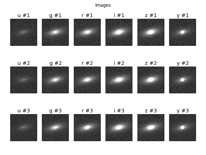
# Plot images
ima = dict(interpolation='nearest', origin='lower', cmap='gray',
           vmin=-5.*pixnoise, vmax=20.*pixnoise)
plt.subplots_adjust(left=0.05, right=0.95, bottom=0.05, top=0.92)
plt.clf()
for i,band in enumerate(bands):
    for e in range(nepochs):
        plt.subplot(nepochs, len(bands), e*len(bands) + i +1)
        plt.imshow(tims[nepochs*i + e].getImage(), **ima)
        plt.xticks([]); plt.yticks([])
        plt.title('%s #%i' % (band, e+1))
plt.suptitle('Images')
plt.savefig('8.png')

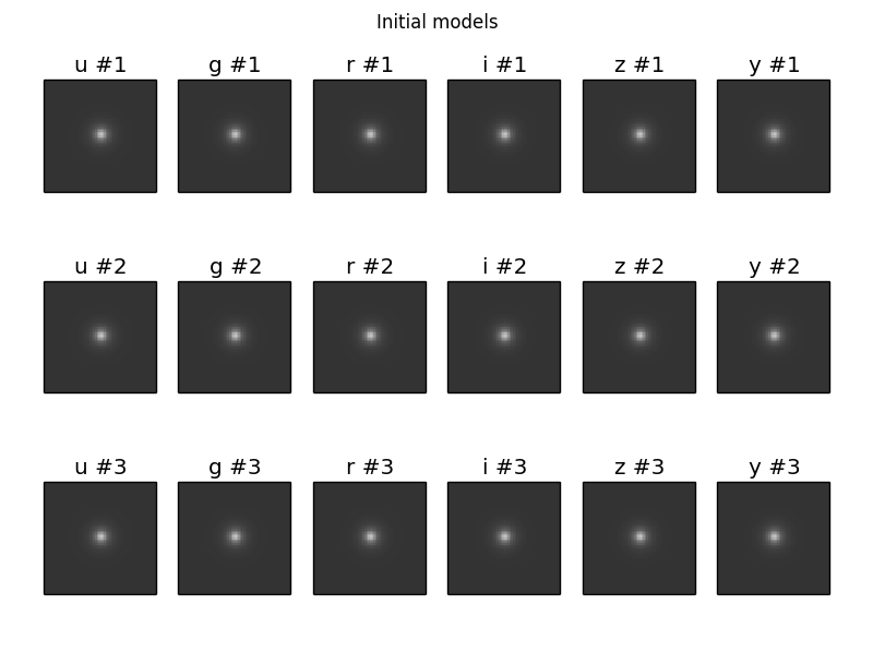
# Plot initial models:
mods = [tractor.getModelImage(i) for i in range(len(tims))]
plt.clf()
for i,band in enumerate(bands):
    for e in range(nepochs):
        plt.subplot(nepochs, len(bands), e*len(bands) + i +1)
        plt.imshow(mods[nepochs*i + e], **ima)
        plt.xticks([]); plt.yticks([])
        plt.title('%s #%i' % (band, e+1))
plt.suptitle('Initial models')
plt.savefig('9.png')

# Freeze all image calibration parameters
tractor.freezeParam('images')

# Take several linearized least squares steps
for i in range(20):
    dlnp,X,alpha = tractor.optimize()
    print 'dlnp', dlnp
    if dlnp < 1e-3:
        break

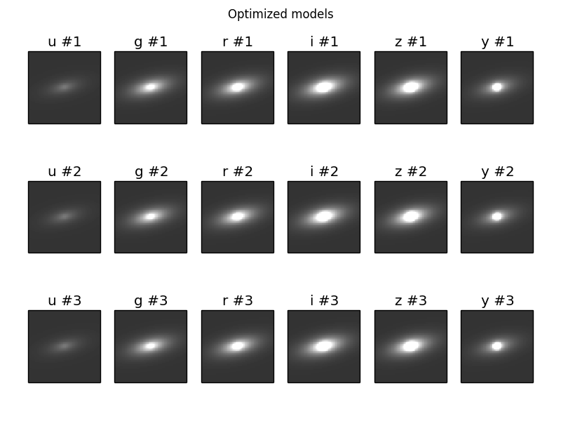
# Plot optimized models:
mods = [tractor.getModelImage(i) for i in range(len(tims))]
plt.clf()
for i,band in enumerate(bands):
    for e in range(nepochs):
        plt.subplot(nepochs, len(bands), e*len(bands) + i +1)
        plt.imshow(mods[nepochs*i + e], **ima)
        plt.xticks([]); plt.yticks([])
        plt.title('%s #%i' % (band, e+1))
plt.suptitle('Optimized models')
plt.savefig('10.png')

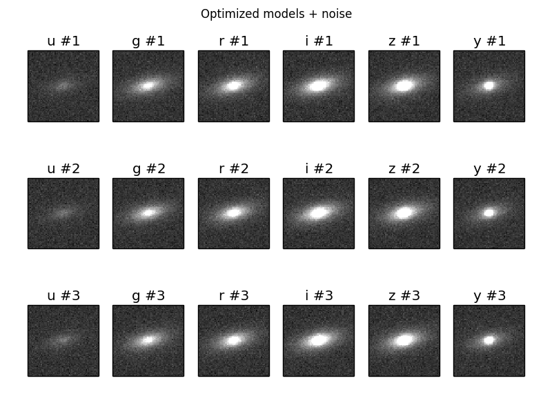
# Plot optimized models + noise:
plt.clf()
for i,band in enumerate(bands):
    for e in range(nepochs):
        plt.subplot(nepochs, len(bands), e*len(bands) + i +1)
        mod = mods[nepochs*i + e]
        plt.imshow(mod + pixnoise * np.random.normal(size=mod.shape), **ima)
        plt.xticks([]); plt.yticks([])
        plt.title('%s #%i' % (band, e+1))
plt.suptitle('Optimized models + noise')
plt.savefig('11.png')

The resulting plots are:

This is our terrible initial guess:

Here are the optimized models:

And here are the optimized models with the expected about of per-pixel noise added.